Jacobian Matrix 考虑$f(x)=x^2$,求导得$\frac{df}{dx}=2x$
当进入多元函数(Multi-Variable Functions),比如$f(x_1, x_2)=x_1^2+3x_1 x_2 +x_2^2$,则:
现在我们定义雅可比矩阵(Jacobian Matrix):
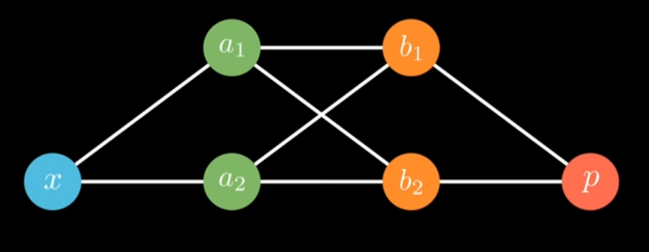
Application: Neural Networks
上面是一个$[1, 2, 2, 1]$的全连接神经网络,我们有以下3个雅可比矩阵:
Code 手动计算
1
2
3
4
5
6
7
8
9
10
11
12
13
14
15
16
17
18
19
20
21
22
23
24
25
26
27
28
29
30
31
32
33
34
35
36
37
38
39
40
41
42
43
44
45
46
47
48
49
50
51
52
53
54
55
56
57
58
59
60
61
62
63
64
65
66
67
68
69
70
71
72
73
74
75
76
77
78
79
80
81
82
83
84
85
86
87
88
89
90
91
92
93
94
95
96
97
98
99
100
101
import torchimport torch.nn as nnfrom torch.autograd.functional import jacobiantorch.manual_seed(0 ) class SmallMLP (nn.Module): def __init__ (self ): super ().__init__() self .l1 = nn.Linear(1 , 2 ) self .l2 = nn.Linear(2 , 2 ) self .l3 = nn.Linear(2 , 1 ) self .act = torch.tanh def forward (self, x ): a = self .act(self .l1(x)) b = self .act(self .l2(a)) p = self .l3(b) return p model = SmallMLP() x0 = torch.tensor([1.0 ]) def layer1 (x ): a = model.act(model.l1(x)) return a def layer2 (a ): b = model.act(model.l2(a)) return b def layer3 (b ): p = model.l3(b).squeeze() return p def whole (x ): a = layer1(x) b = layer2(a) p = layer3(b) return p J1 = jacobian(layer1, x0, create_graph=False ) a0 = layer1(x0).detach() J2 = jacobian(layer2, a0, create_graph=False ) b0 = layer2(a0).detach() J3 = jacobian(layer3, b0, create_graph=False ) print ("J1 (d a / d x) shape:" , J1.shape)print (J1)print ("J2 (d b / d a) shape:" , J2.shape)print (J2)print ("J3 (d p / d b) shape:" , J3.shape)print (J3)dp_dx = jacobian(whole, x0, create_graph=False ) print ("dp/dx (from whole network):" , dp_dx)J1_mat = J1 J2_mat = J2 J3_mat = J3 dp_dx_chain = J3_mat @ J2_mat @ J1_mat print ("dp/dx from J3*J2*J1:" , dp_dx_chain)print ("difference:" , dp_dx_chain.item() - dp_dx.item())
1
2
3
4
5
6
7
8
9
10
11
J1 (d a / d x) shape: torch.Size([2, 1]) tensor([[-0.0040], [ 0.5156]]) J2 (d b / d a) shape: torch.Size([2, 2]) tensor([[-0.2704, 0.1882], [-0.0139, 0.5565]]) J3 (d p / d b) shape: torch.Size([2]) tensor([-0.2137, -0.1390]) dp/dx (from whole network): tensor([-0.0609]) dp/dx from J3*J2*J1: tensor([-0.0609]) difference: 0.0
使用自动微分
1 2 3 4 5 6 7 8 9 10 11 12 x = torch.tensor([1.0 ], requires_grad=True ) p = model(x) p.backward() print ("dp/dx (from autograd backward):" , x.grad.item())print ("difference:" , x.grad.item() - dp_dx.item())
1
2
dp/dx (from autograd backward): -0.060868293046951294 difference: 0.0