Note
对于PINN,通常损失有基本的两项构成,物理损失和边界损失:
$$\mathcal{L}(\theta) = \mathcal{L}_p(\theta) + \mathcal{L}_b(\theta),$$
二者有以下形式:
$$\mathcal{L}p(\theta) = \frac{1}{N_p} \sum{i}^{N_p} | \mathcal{D}[NN(x_i; \theta); \lambda] - f(x_i) |^2,$$ $$\mathcal{L}b(\theta) = \sum{k} \frac{1}{N_{bk}} \sum_{j}^{N_{bk}} | \mathcal{B}k[NN(x{kj}; \theta)] - g_k(x_{kj}) |^2,$$
上面这种称为软约束,在实际训练中二者通常有冲突,并且调整二者的权重系数也是个繁琐的工作。对此,可以将边界条件直接融入近似解,作为其中必然满足的一部分,如对于波动方程:
$$\left[ \nabla^2 - \frac{1}{c^2} \frac{\partial^2}{\partial t^2} \right] u(x, t) = f(x, t),$$ $$u(x, 0) = g_1(x),$$ $$\frac{\partial u}{\partial t}(x, 0) = g_2(x),$$
可以假设近似解的形式为:
$$\hat{u}(x, t; \theta) = g_1(x) + t,g_2(x) + t^2,NN(x, t; \theta)$$
如此,在$t=0$时,解强制满足$g_1(x)$,在对$t$求导后,$t=0$时也强制满足$g_2(x)$,如此损失只需包含物理损失$\mathcal{L}_p(\theta)$,变为简单的无约束优化问题。
考虑一维示例:
$$\frac{du}{dx} = \cos(\omega x),$$ $$u(0) = 0,$$
这个方程有精确解:
$$u(x) = \frac{1}{\omega} \sin(\omega x)$$
我们设计近似解为:
$$\hat{u}(x; \theta) = \tanh(\omega x) NN(x; \theta)$$
这里$x=0$时,$tanh(\omega x)=0$,并且在远离边界$x=0$的地方,其值趋向于$\pm 1$,这样神经网络就无需对该函数进行大量补偿。最终PINN使用的损失函数为:
$$\mathcal{L}(\theta) = \mathcal{L}p(\theta) = \frac{1}{N_p} \sum{i}^{N_p} \left| \frac{d}{dx} \hat{u}(x_i; \theta) - \cos(\omega x_i) \right|^2$$
首先对低频情况$\omega = 1$进行训练,使用2个隐藏层,每层16个神经元和tanh激活函数的全连接网络,在$x \in [-2\pi, 2\pi]$上均匀分布200个训练点,在$x$进入网络之前,会归一化到$[-1, 1]$,而为了匹配精确解的幅值区域,会让输出乘以$\frac{1}{\omega}$。
在高频案例$\omega = 15$中,训练点增加到3000,并采取了3种不同的网络结构配置,最终预测结果与损失下降如下图所示。
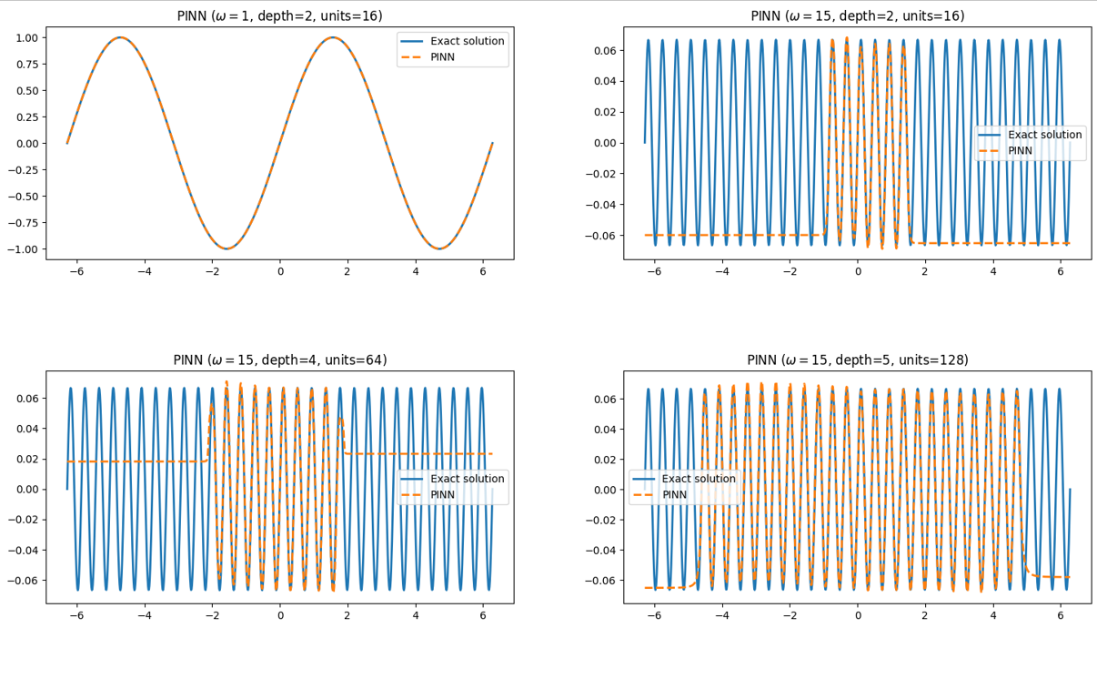
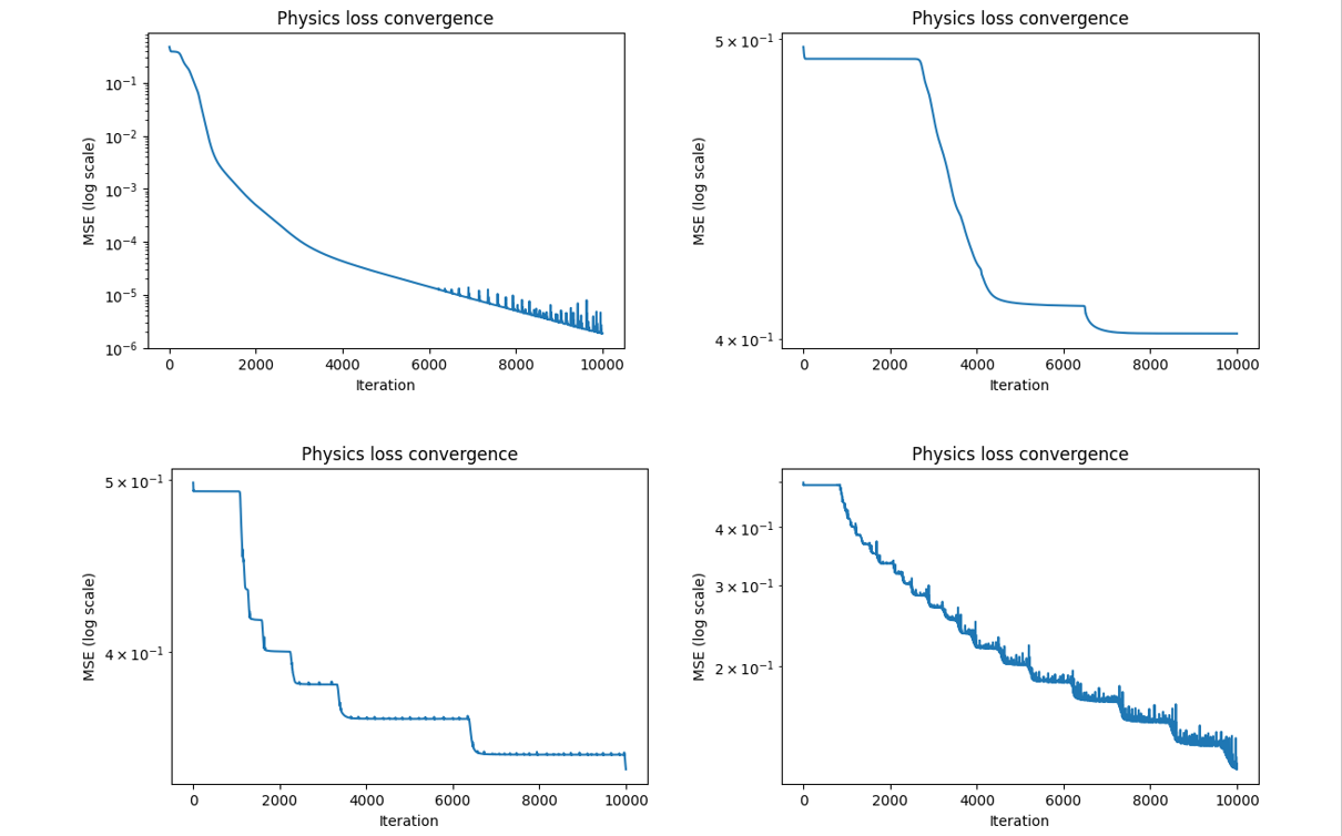
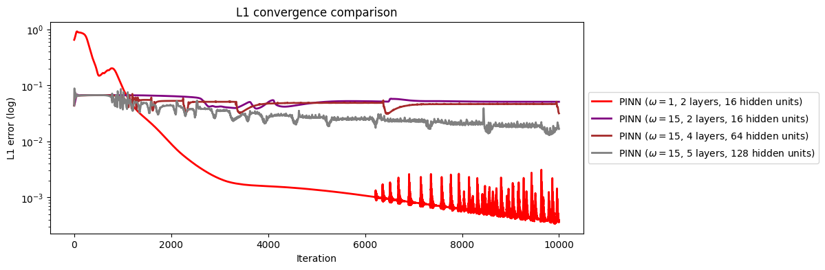
虽然PINN在低频表现良好,但高频面临巨大困难,要学习高频需要大量参数,且收敛缓慢,精度低。对于该问题,向更高频率扩展等同于向更大的域尺寸扩展,因为我们在把$x$输入网络前已经归一化到$[-1, 1]$,所以保持$\omega = 1$不变,同时将域尺寸扩大15倍并重新归一化,与直接将$\omega = 15$对于优化来说是一样的。这就引出了FB-PINN。下图是四种情况的$L1$误差对比。
Code
完整代码实现:
1
2
3
4
5
6
7
8
9
10
11
12
13
14
15
16
17
18
19
20
21
22
23
24
25
26
27
28
29
30
31
32
33
34
35
36
37
38
39
40
41
42
43
44
45
46
47
48
49
50
51
52
53
54
55
56
57
58
59
60
61
62
63
64
65
66
67
68
69
70
71
72
73
74
75
76
77
78
79
80
81
82
83
84
85
86
87
88
89
90
91
92
93
94
95
96
97
98
99
100
101
102
103
104
105
106
107
108
109
110
111
112
113
114
115
116
117
118
119
120
121
122
123
124
125
126
127
128
129
130
131
132
133
134
| import numpy as np
import matplotlib.pyplot as plt
import torch
import torch.nn as nn
device = torch.device('cuda' if torch.cuda.is_available() else 'cpu')
omega = 15
units = 128
depth = 5
train_num = 3000
class Net(nn.Module):
def __init__(self, in_dim=1, out_dim=1, units=128, depth=5):
super().__init__()
layers = []
layers.append(nn.Linear(in_dim, units))
layers.append(nn.Tanh())
for _ in range(depth - 1):
layers.append(nn.Linear(units, units))
layers.append(nn.Tanh())
layers.append(nn.Linear(units, out_dim))
self.net = nn.Sequential(*layers)
def forward(self, x_norm):
return self.net(x_norm)
model = Net(in_dim=1, out_dim=1, units=units, depth=depth).to(device)
xmin = -2*np.pi
xmax = 2*np.pi
x = np.linspace(xmin, xmax, train_num).reshape(-1, 1)
x = torch.tensor(x, dtype=torch.float32, requires_grad=True).to(device)
x_eval = torch.linspace(xmin, xmax, 5000).reshape(-1, 1).to(device)
def normalize_x(x):
return 2.0 * (x - xmin) / (xmax - xmin) - 1.0
def u_hat(x):
x_norm = normalize_x(x)
nn_out = model(x_norm)
nn_out = (1.0/omega) * nn_out
return torch.tanh(omega * x) * nn_out
def dudx(x):
x.requires_grad_(True)
u = u_hat(x)
du_dx = torch.autograd.grad(
u, x,
grad_outputs=torch.ones_like(u),
create_graph=True
)[0]
return du_dx
def u_exact(x):
return (1.0/omega) * torch.sin(omega * x)
optimizer = torch.optim.Adam(model.parameters(), lr=1e-3)
loss_history = []
l1_history = []
epochs = 10000
for epoch in range(epochs):
optimizer.zero_grad()
pred = dudx(x)
target = torch.cos(omega * x)
loss = torch.mean((pred - target)**2)
loss.backward()
optimizer.step()
loss_history.append(loss.item())
with torch.no_grad():
u_pred_eval = u_hat(x_eval)
u_true_eval = u_exact(x_eval)
l1 = torch.mean(torch.abs(u_pred_eval - u_true_eval)).item()
l1_history.append(l1)
if epoch % 500 == 0:
print(f"Iter {epoch}/{epochs}, Loss = {loss.item():.6e}, L1 = {l1:.6e}")
l1_array = np.array(l1_history)
np.savetxt(f"L1_omega{omega}_units{units}_depth{depth}.txt", l1_array)
x_test = torch.linspace(xmin, xmax, 1000).reshape(-1,1).to(device)
u_pinn = u_hat(x_test).detach().cpu().numpy()
u_real = u_exact(x_test).detach().cpu().numpy()
x_test_np = x_test.detach().cpu().numpy()
plt.figure(figsize=(8,4))
plt.plot(x_test_np, u_real, label="Exact solution", linewidth=2)
plt.plot(x_test_np, u_pinn, '--', label="PINN", linewidth=2)
plt.legend()
plt.title(rf"PINN ($\omega = {omega}$, depth={depth}, units={units})")
plt.show()
plt.figure(figsize=(6,4))
plt.plot(loss_history)
plt.yscale("log")
plt.xlabel("Iteration")
plt.ylabel("MSE (log scale)")
plt.title("Physics loss convergence")
plt.show()
plt.figure(figsize=(6,4))
plt.plot(l1_history)
plt.yscale("log")
plt.xlabel("Iteration")
plt.ylabel("L1 error (log scale)")
plt.title("L1 convergence (5000 eval points)")
plt.show()
|
注意3个关键函数,u_hat用于给出我们假设的近似解,归一化也在内部进行,尽管给网络输入的是x_norm,但求导时对象是x,如此根据链式法则,PDE方程就不会更改。
1
2
3
4
5
6
7
8
9
10
11
12
13
14
15
16
17
18
| def normalize_x(x):
return 2.0 * (x - xmin) / (xmax - xmin) - 1.0
def u_hat(x):
x_norm = normalize_x(x)
nn_out = model(x_norm)
nn_out = (1.0/omega) * nn_out
return torch.tanh(omega * x) * nn_out
def dudx(x):
x.requires_grad_(True)
u = u_hat(x)
du_dx = torch.autograd.grad(
u, x,
grad_outputs=torch.ones_like(u),
create_graph=True
)[0]
return du_dx
|
误差图对比:
1
2
3
4
5
6
7
8
9
10
11
12
13
14
15
16
17
18
19
20
21
22
23
24
25
26
27
28
29
30
31
32
33
34
35
36
37
38
39
40
41
42
43
44
45
46
47
48
49
| import numpy as np
import matplotlib.pyplot as plt
files = [
"L1_omega1_units16_depth2.txt",
"L1_omega15_units16_depth2.txt",
"L1_omega15_units64_depth4.txt",
"L1_omega15_units128_depth5.txt",
]
labels = [
"PINN ($\\omega = 1$, 2 layers, 16 hidden units)",
"PINN ($\\omega = 15$, 2 layers, 16 hidden units)",
"PINN ($\\omega = 15$, 4 layers, 64 hidden units)",
"PINN ($\\omega = 15$, 5 layers, 128 hidden units)",
]
colors = ["red", "purple", "brown", "gray"]
plt.figure(figsize=(10,4))
for f, lab, c in zip(files, labels, colors):
l1 = np.loadtxt(f)
plt.plot(l1, label=lab, linewidth=2, color=c)
plt.yscale("log")
plt.xlabel("Iteration")
plt.ylabel("L1 error (log)")
plt.legend(
fontsize=10,
loc='center left',
bbox_to_anchor=(1, 0.5)
)
plt.title("L1 convergence comparison")
plt.show()
|
Reference
Finite basis physics-informed neural networks (FBPINNs): a scalable domain decomposition approach for solving differential equations | Advances in Computational Mathematics