FNO,是继PINN后一种用“算子学习”的方式求解PDE的方法,全名为傅里叶神经算子(Fourier Neural Operator)。https://arxiv.org/pdf/2010.08895 https://github.com/lu-group/deeponet-fno/tree/main?tab=readme-ov-file
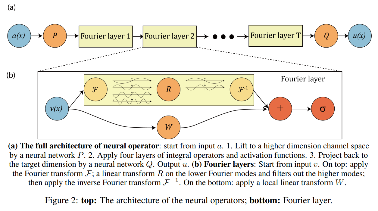
上图为FNO的网络结构,我们从最简单的一维瞬态的 Burger’s Equation 开始上手,控制方程如下:
这里的算子学习就是学习一组初始条件对应的解,神经网络的输入是$u(x,t=0)=u_o(x)$,输出是$u=u(x,t=1)$,因此神经网络学习的算子$G$可以表示为:
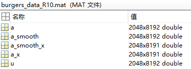
数据准备 训练数据集是用matlab生成的,如下图所示:
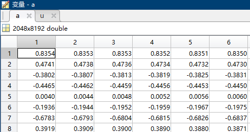
$u_0(x)$和$u(x,t=1)$就是这里的$a$和$u$,$(2048x8192)$表示有2048组不同的初始条件,每组有8192个$x$的值,这里使用了平均采样,即x = linspace(0,1,8192)。
上图就是0时刻在位置$(0,1)$上对应$u(x,t)$的值,注意不是$x$的值,故有正有负。
数据集的生成对于最终结果以及网络的泛化性能可能有重要的影响,这里使用了随机采样方法,核心思想是高斯随机场,这里不展开讲。
源码分析 源码有三大部分,主函数FNO_main,神经网络类class FNO1d,以及傅里叶层class SpectralConv1d,首先来看主函数。
FNO_main的使用:
1
2
3
4
5
6
if __name__ == "__main__" : training_data_resolution = 128 save_index = 0 FNO_main(training_data_resolution, save_index)
基本参数 1 2 3 4 5 6 7 8 9 10 11 12 13 14 15 16 ntrain = 1000 ntest = 200 s = train_data_res sub = 2 **13 // s batch_size = 20 learning_rate = 0.001 epochs = 500 step_size = 100 gamma = 0.5 modes = 16 width = 64
读入数据&数据处理 从 .mat 文件读入数据 -> 降采样 -> 分成训练集和测试集
1 2 3 4 5 6 7 8 dataloader = MatReader('burgers_data_R10.mat' ) x_data = dataloader.read_field('a' )[:,::sub] y_data = dataloader.read_field('u' )[:,::sub] x_train = x_data[:ntrain,:] y_train = y_data[:ntrain,:] x_test = x_data[-ntest:,:] y_test = y_data[-ntest:,:]
x_data,y_data只包括$u(x,t)$的数值,2048组初始条件,取了1000组作为训练集,200组作为测试集,下面生成了网格位置$x$的数据,与$u$拼接在一起,最终形成一个维度 (1000, 128, 2) 的数据集作为整体输入,训练的时候一批的大小为 (batch_size=20, 128, 2),最后一个维度的两个数分别为该位置初始时刻的大小以及该位置的坐标。
1 2 3 4 5 6 7 8 9 10 grid_all = np.linspace(0 , 1 , 2 **13 ).reshape(2 **13 , 1 ).astype(np.float64) grid = grid_all[::sub,:] grid = torch.tensor(grid, dtype=torch.float ) x_train = torch.cat([x_train.reshape(ntrain,s,1 ), grid.repeat(ntrain,1 ,1 )], dim=2 ) x_test = torch.cat([x_test.reshape(ntest,s,1 ), grid.repeat(ntest,1 ,1 )], dim=2 ) train_loader = torch.utils.data.DataLoader(torch.utils.data.TensorDataset(x_train, y_train), batch_size=batch_size, shuffle=True ) test_loader = torch.utils.data.DataLoader(torch.utils.data.TensorDataset(x_test, y_test), batch_size=batch_size, shuffle=False )
grid.repeat(ntrain,1,1) 就是在 dim = 0这个维度(不同样本的维度)进行重复,简单来说就是使得 grid[x, a, b] = grid[y, a, b]。
class FNO1d 1 2 3 4 5 6 7 8 9 10 11 12 13 14 15 16 17 18 19 20 21 22 23 24 25 26 27 28 29 30 31 32 33 34 35 36 37 38 39 40 class FNO1d (nn.Module): def __init__ (self, modes, width ): super (FNO1d, self ).__init__() """ The overall network. It contains 4 layers of the Fourier layer. 1. Lift the input to the desire channel dimension by self.fc0 . 2. 4 layers of the integral operators u' = (W + K)(u). W defined by self.w; K defined by self.conv . 3. Project from the channel space to the output space by self.fc1 and self.fc2 . input: the solution of the initial condition and location (a(x), x) input shape: (batchsize, x=s, c=2) output: the solution of a later timestep output shape: (batchsize, x=s, c=1) """ self .modes1 = modes self .width = width self .fc0 = nn.Linear(2 , self .width) """ 输入时的维度是(20, 128, 2), 其中第一个维度20指的是 batch_size=20。 通过 self.fc0 = nn.Linear(2, self.width=64) 后维度变为 (20, 128, 64)。这一步是 position-wise 的,即对于每一个(a(x), x)对单独操作。 """ self .conv0 = SpectralConv1d(self .width, self .width, self .modes1) self .conv1 = SpectralConv1d(self .width, self .width, self .modes1) self .conv2 = SpectralConv1d(self .width, self .width, self .modes1) self .conv3 = SpectralConv1d(self .width, self .width, self .modes1) self .w0 = nn.Conv1d(self .width, self .width, 1 ) self .w1 = nn.Conv1d(self .width, self .width, 1 ) self .w2 = nn.Conv1d(self .width, self .width, 1 ) self .w3 = nn.Conv1d(self .width, self .width, 1 ) self .fc1 = nn.Linear(self .width, 128 ) self .fc2 = nn.Linear(128 , 1 )
具体神经网络输入时的维度是(20, 128, 2),其中第一个维度20指的是 batch_size=20。这里通过fc0的升维操作变成 (20, 128, 64)。既达到了和网格数量多少无关,又提高了维度,这一步也是 FNO 输入与网格粗细无关的重要一环(另一环和傅立叶变换后取固定长度模式有关)。
提升维度有两个好处:
因为目前维度(128, 2)的特征不过是一个更高维度的函数空间在有限维度的投影,目前这个长度可能不足以表征原始函数空间到另一个函数空间的映射(或者说不能在要求的精度下完成),因此这一步操作把特征的长度扩充到了(128, 64),之后的神经网络变换都在这个大小基础上进行(在更接近原来函数空间的一个高维空间进行),能够学习到更复杂的变换,最后再投影回低维度。
保持第一个维度128不变。一方面这样可以做到和网格粗细无关,另一方面也是考虑到后续的傅立叶变换。因为第一个维度是有物理意义的,它是和位置/网格直接关联的,对这个维度进行傅立叶变换是一个更有物理意义的操作(后续有一个permute操作),倘若再这个维度进行升维,就失去了原有的物理意义(到了一个更抽象的高维空间,对它进行傅立叶变换的话可能可行,但很难讲出道理)。
最后从forward函数看看整体流程:
1 2 3 4 5 6 7 8 9 10 11 12 13 14 15 16 17 18 19 20 21 22 23 24 25 26 27 28 29 30 31 32 33 34 def forward (self, x ): x = self .fc0(x) x = x.permute(0 , 2 , 1 ) """ torch.permute 其实就是对数组不同维度进行变换,本例的结果就会导致 x'[a, b, c] = x[a, c, b], 那么维度也随之从原来的(20, 128, 64)变为(20, 64, 128),之所以做这个变换也是因为之后的傅立叶变换 是针对长度为128的那个和位置相关的维度, 而人们习惯于操作最后一个维度, 因此把这个维度变换到最后一维。 """ x1 = self .conv0(x) x2 = self .w0(x) x = x1 + x2 x = F.relu(x) x1 = self .conv1(x) x2 = self .w1(x) x = x1 + x2 x = F.relu(x) x1 = self .conv2(x) x2 = self .w2(x) x = x1 + x2 x = F.relu(x) x1 = self .conv3(x) x2 = self .w3(x) x = x1 + x2 x = x.permute(0 , 2 , 1 ) x = self .fc1(x) x = F.relu(x) x = self .fc2(x) return x
可以看到升维和降维之间有4个傅里叶层:
1 2 3 4 x1 = self .conv0(x) x2 = self .w0(x) x = x1 + x2 x = F.relu(x)
与前面网络结构图展示的一致,一个傅里叶块包括一个傅里叶层和一个偏置,其中偏置是一个一维卷基层,输入通道输和输出通道数相等为width=64,卷积核大小为1x1。二者相加,再有一个激活函数。
class SpectralConv1d 下面是傅里叶层的具体实现:
1 2 3 4 5 6 7 8 9 10 11 12 13 14 15 16 17 18 19 20 21 22 23 24 25 26 27 28 29 30 31 32 33 class SpectralConv1d (nn.Module): def __init__ (self, in_channels, out_channels, modes1 ): super (SpectralConv1d, self ).__init__() """ 1D Fourier layer. It does FFT, linear transform, and Inverse FFT. """ self .in_channels = in_channels self .out_channels = out_channels self .modes1 = modes1 self .scale = (1 / (in_channels*out_channels)) self .weights1 = nn.Parameter(self .scale * torch.rand(in_channels, out_channels, self .modes1, dtype=torch.cfloat)) def compl_mul1d (self, input , weights ): return torch.einsum("bix,iox->box" , input , weights) def forward (self, x ): batchsize = x.shape[0 ] x_ft = torch.fft.rfft(x) out_ft = torch.zeros(batchsize, self .out_channels, x.size(-1 )//2 + 1 , device=x.device, dtype=torch.cfloat) out_ft[:, :, :self .modes1] = self .compl_mul1d(x_ft[:, :, :self .modes1], self .weights1) x = torch.fft.irfft(out_ft, n=x.size(-1 )) return x
self.weights1权重维数为(64, 64, 16),最后一个维度是傅立叶变换截断的阶数16。
傅立叶层的一部分其实就像是频域做了一次全连接,不管输入多长,变换到频域后总是取前16个进行变换再反变换,因此和长度/网格粗细无关。
优化器 1 2 optimizer = torch.optim.Adam(model.parameters(), lr=learning_rate, weight_decay=1e-4 ) scheduler = torch.optim.lr_scheduler.StepLR(optimizer, step_size=step_size, gamma=gamma)
使用Adam算法,并每过 step_size个epoch就让学习率乘一个gamma作衰减。
utilities 代码引入了三个自定义函数(类),MatReader、count_params、LpLoss,这里做简要介绍。
MatReader类用于读取.mat数据。
LpLoss用于计算$L_p$范数损失,这里采用$L_2$损失,可选相对误差与绝对误差。
count_params用于计算任意神经网络模型的参数量,挺有意思的泛用性函数。
1 2 3 4 5 def count_params (model ): c = 0 for p in list (model.parameters()): c += reduce(operator.mul, list (p.size())) return c
测试结果 一次训练结果的输出如下,可以看到,使用傅里叶变换,计算都变成乘法,速度很快,误差也在1%左右:
1 2 3 4 5 6 Epoch: 499 , time: 0.188 , Train Loss: 6.387e-05 , Train l2: 0.0108 , Test l2: 0.0117 ============================= Training done... Training time: 95.983 =============================
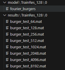
保存了模型,并生成了不同分辨率下的测试集
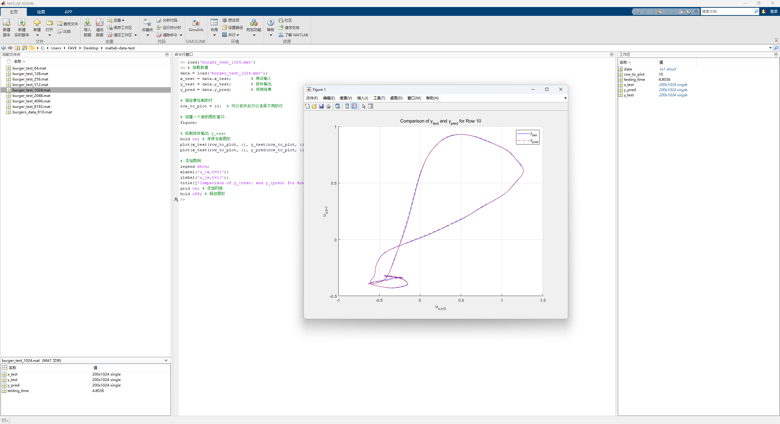
绘制结果matlab代码:
1 2 3 4 5 6 7 8 9 10 11 12 13 14 15 16 17 18 19 20 21 22 23 24 data = load('burger_test_1024.mat' ); x_test = data.x_test; y_test = data.y_test; y_pred = data.y_pred; row_to_plot = 10 ; figure ;hold on; plot (x_test(row_to_plot, :), y_test(row_to_plot, :), 'b-' , 'DisplayName' , 'y_{test}' ); plot (x_test(row_to_plot, :), y_pred(row_to_plot, :), 'r--' , 'DisplayName' , 'y_{pred}' ); legend show;xlabel('u_{x,t=0}' ); ylabel('u_{x,t=1}' ); title(['Comparison of y_{test} and y_{pred} for Row ' num2str(row_to_plot)]); grid on; hold off;
测试横坐标是0s的u,纵坐标是1s的u